

In today’s data-driven world, making informed business decisions is crucial for success. One effective way to visualize your data and track key performance indicators (KPIs) is by building an Excel dashboard. This guide will help business owners and Excel users create their first KPI dashboard, enhancing their ability to make strategic decisions based on business analytics and data visualization.
Why Use a KPI Dashboard?
A KPI dashboard provides a visual representation of your data, allowing you to:
– Monitor performance: Track sales performance, marketing effectiveness, and operational efficiency.
– Identify trends: Spot patterns and trends over time to make informed decisions.
– Simplify reporting: Transform complex data sets into easy-to-understand visuals.
– Enhance communication: Share insights with stakeholders more effectively.
Step 1: Define Your Objectives
Before diving into Excel, it’s essential to determine what you want to achieve with your dashboard. Consider the following questions:
1. What are the key metrics? Identify the KPIs that matter most to your business.
2. Who is the audience? Understand who will be using the dashboard and tailor it to their needs.
3. What decisions will it support? Ensure your dashboard aligns with your business objectives.
Step 2: Collect and Prepare Your Data
Having accurate and well-structured data is crucial for effective business intelligence. Here’s how to get started:
– Gather Data: Collect data from various sources, such as sales reports, marketing campaigns, and customer feedback.
– Clean Data: Remove duplicates, fill in missing values, and standardize formats to ensure consistency.
– Use Power Query: Excel’s Power Query can help automate data cleaning and transformation. To do this:
– Go to the Data tab.
– Select Get Data > From File > From Workbook.
– Load and transform your data as needed.
Step 3: Create a Data Model
Once your data is organized, it’s time to create a data model that facilitates analysis. This involves:
– Using Tables: Convert your data ranges into Excel tables by selecting your data and pressing Ctrl + T. This helps in managing data more effectively.
– Creating Relationships: If you’re working with multiple tables, establish relationships between them using the Manage Relationships option under the Data tab.
Step 4: Build PivotTables
PivotTables are a powerful feature in Excel that allows you to summarize and analyze data quickly. Here’s how to create one:
1. Insert a PivotTable:
– Select your data table.
– Go to the Insert tab and click on PivotTable.
– Choose where you want the PivotTable to be placed (new worksheet or existing one).
2. Configure Your PivotTable:
– Drag and drop fields into the Rows, Columns, and Values areas to structure your data.
– Use filters to focus on specific data points relevant to your KPIs.
Step 5: Visualize Your Data
Data visualization is key to making insights accessible. Here are some visualization techniques to consider:
– Charts: Use bar charts, line graphs, or pie charts to display trends and comparisons.
– Conditional Formatting: Highlight critical data points using Excel’s conditional formatting tools.
– Slicers: Add slicers to allow users to filter data easily and interactively.
Step 6: Create Your KPI Dashboard
Now that you have your data model and visualizations ready, it’s time to assemble your KPI dashboard. Follow these steps:
1. Choose a Layout: Decide on a logical layout that groups related KPIs together. Consider using a grid format for clarity.
2. Insert Visualizations:
– Go to the dashboard sheet.
– Copy and paste your charts and tables from the PivotTables.
3. Add Interactivity:
– Include slicers and drop-down menus to allow users to filter and interact with the data.
– Use hyperlinks to navigate between different sections of your dashboard if needed.
Step 7: Test and Refine
Before presenting your dashboard, test it thoroughly. Consider the following:
– User Experience: Ensure that the dashboard is intuitive and easy to navigate.
– Accuracy: Double-check calculations and data sources to confirm accuracy.
– Feedback: Gather input from potential users and make adjustments based on their suggestions.
Step 8: Share Your Dashboard
Once your KPI dashboard is ready, it’s time to share it with stakeholders. You can:
– Export as PDF: For a static report, export your dashboard as a PDF.
– Share the Workbook: If real-time interaction is needed, share the Excel workbook directly.
– Use Excel Online: For collaborative efforts, use Excel Online to allow multiple users to view and edit simultaneously.
Conclusion
Creating a KPI dashboard in Excel is a powerful way to leverage your data for data-driven decisions. By following this practical guide, business owners and Excel users can transform their raw data into actionable insights. Remember, the key to success lies in defining clear objectives, preparing accurate data, and continuously refining your dashboard based on feedback.
As you embark on this journey towards better business intelligence, keep experimenting with different visualizations and data sources. The more you explore, the more effective your KPI dashboard will become in supporting your business goals.
—
By implementing these steps, you’ll be on your way to mastering the art of Excel dashboards and making impactful business decisions based on solid data analytics. Happy dashboarding!
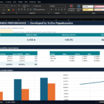
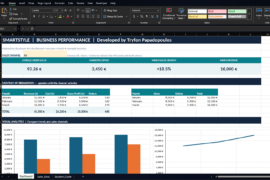
Practical Example: From Excel Data to Better Business Decisions

Δοκιμάστε τον live (σε κανονική λειτουργία real time)
—



Comments are closed.