#excel_tips #transpose #softexperia


Filter employees by department in columns from mixed data Function for cell A7 =FILTER($G7:$G$33;$H$7:$H$33=A6) Function for cell B7 =FILTER($G7:$G$33;$H$7:$H$33=B6) Music track: A Positive Direction by Aylex Source: https://freetouse.com/music Royalty Free Music for Video (Safe) #mindstormGR #dynamic_filters #excel #educational


I find staircases endlessly inspiring, such a perfect opportunity for building a character in life. They teach you that you have to deal with your ups and downs if you want to make it work. Άνοδος και κάθοδος Με εμπνέουν οι σκάλες. Είναι μια τέλεια ευκαιρία για να γίνεις λίγο καλύτερος. Σε μαθαίνουν ότι πρέπει να αντιμετωπίσεις πρώτα τα δικά σου τα πάνω και τα κάτω. Πρέπει και να ανέβεις και να κατέβεις. Να βρεις τα πατήματά σου και τις ανάσες σου. Διαφορετικά δεν θα βρεις ούτε το σωστό σχέδιο ούτε το σωστό ρυθμό, και έτσι δεν θα μπορέσεις ούτε να δημιουργήσεις κάτι, ούτε να εμπνεύσεις κάποιον σ’ αυτήν τη ζωή. #mindstormGR
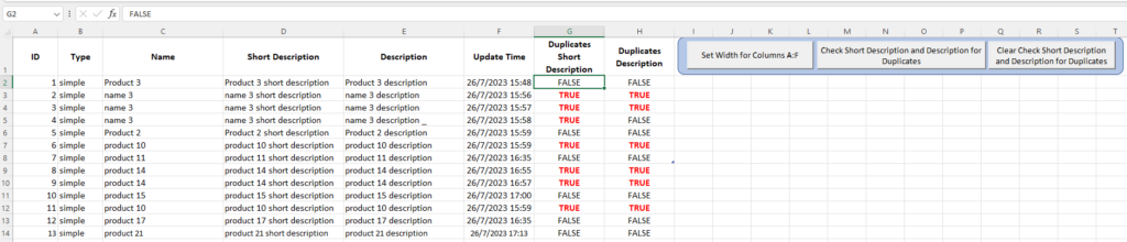


Rules 1) If Sales >= 20000, then 4% commission 2) If Sales >= 5000 and < 20000, then 5% commission 3) If Sales >= 1 and < 5000, then 6% commission D3 cell function =IF(C3>=$G$3;$H$3;IF(C3>=$G$4;$H$4;$H$5))*C3 D4 cell function =IF(C4>=$G$3;$H$3;IF(C4>=$G$4;$H$4;$H$5))*C4 D5 cell function =IF(C5>=$G$3;$H$3;IF(C5>=$G$4;$H$4;$H$5))*C5 D6 cell function =IF(C6>=$G$3;$H$3;IF(C6>=$G$4;$H$4;$H$5))*C6 Δείτε το σχετικό άρθρο στο blog της ιστοσελίδας softexperia.com . . .

Did you know you can use Python code to create an Excel Data Entry Form and avoid duplicate records? Πώς να δημιουργήσετε μια φόρμα εισαγωγής δεδομένων σε 10 λεπτά με τη γλώσσα προγραμματισμού PYTHON (No VBA) Πώς να διασφαλίσετε ότι δεν θα κάνετε διπλοεγγραφές Excel fields : Name, City, Favorite Color, German, Spanish, English, Children Excel before data entry Data entry form Excel after data entry ‘Python code starts here. import PySimpleGUI as sg import pandas as pd # Add some color to the window sg.theme(‘DarkTeal9’) EXCEL_FILE = ‘data_entry.xlsx’ df = pd.read_excel(EXCEL_FILE) layout = [ [sg.Text(‘Please fill out the following fields:’)], [sg.Text(‘Name’, size=(15,1)), sg.InputText(key=’Name’)], [sg.Text(‘City’, size=(15,1)), sg.InputText(key=’City’)], [sg.Text(‘Favorite Color’, size=(15,1)), sg.Combo([‘Green’, ‘Blue’, ‘Red’], key=’Favorite Color’)], [sg.Text(‘I speak’, size=(15,1)), sg.Checkbox(‘German’, key=’German’), sg.Checkbox(‘Spanish’, key=’Spanish’), sg.Checkbox(‘English’, key=’English’)], [sg.Text(‘No. of Children’, size=(15,1)), sg.Spin([i for i in range(0,16)], initial_value=0, key=’Children’)], [sg.Submit(), sg.Button(‘Clear’), sg.Exit()] ] window = sg.Window(‘Simple data entry form’, layout) def clear_input(): for key…



Overdose of technology Overdose of terminology Overdose of methology Overdose of anxiety Overdose of solitude Overdose of medicine Overdose of detection Overdose of destruction Overdose of pollution Overdose of communication No dose of apology No dose of affection No dose of direction No dose of connection Is there any hope of salvation? #mindstormGR / www.mindstorm.gr


As Greeks all over the world mark International Greek Language Day on February 9, many recall the speeches in English — peppered with Greek-origin words and phrases — given by economist and politician Xenophon Zolotas in the late 1950s. Zolotas was director of the Bank of Greece when he appeared in front of an audience at an International Bank for Reconstruction and Development conference in 1959. He delivered two speeches in English using Greek words to emphasize the wealth of the Greek language and the fact that countless Greek words enrich English. Greek remains a language which greatly enriches international scientific discourse; more than any other, it is the language which developed, shaped and expressed the beginning of most scientific theories, philosophical thoughts, and literature in most of the modern-day languages of the Western world. Here is the second speech delivered Oct. 2, 1959: Kyrie, It is Zeus’ anathema on…

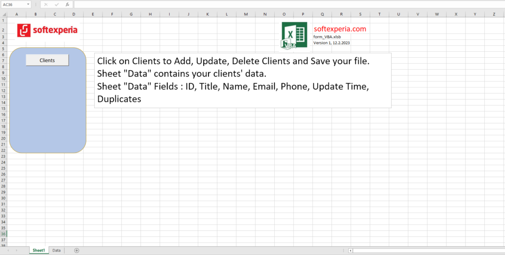

Wordpress Debugging – Δείτε πως να απενεργοποιείτε όλα τα plugins μέσω FTP ή File Manager χωρίς να τα σβήνετε, προκειμένου στη συνέχεια να τα ενεργοποιήσετε ένα ένα και να κάνετε τους ελέγχους συμβατότητας/λειτουργίας που επιθυμείτε. How to reset your plugins folder via FTP or the file manager provided in your host’s control panel. This method preserves plugin options but requires plugins be manually reactivated. Via FTP or your host’s file manager, navigate to the wp-contents folder (directory) – Πας στον κατάλογο wp-content Via FTP or your host’s file manager, rename the folder “plugins” to “plugins.hold” – Μετονομάζεις τον κατάλογο plugins σε plugins.hold Login to your WordPress administration plugins page (/wp-admin/plugins.php) – this will disable any plugin that is “missing”. – Πληκτρολογείς το url demowebsite.com.gr/wp-admin/plugins.php και βλέπεις τη σχετική σελίδα που σου λέει ότι όλα τα plugins είναι απενεργοποιημένα. Via FTP or your host’s file manager, rename “plugins.hold” back to “plugins”…
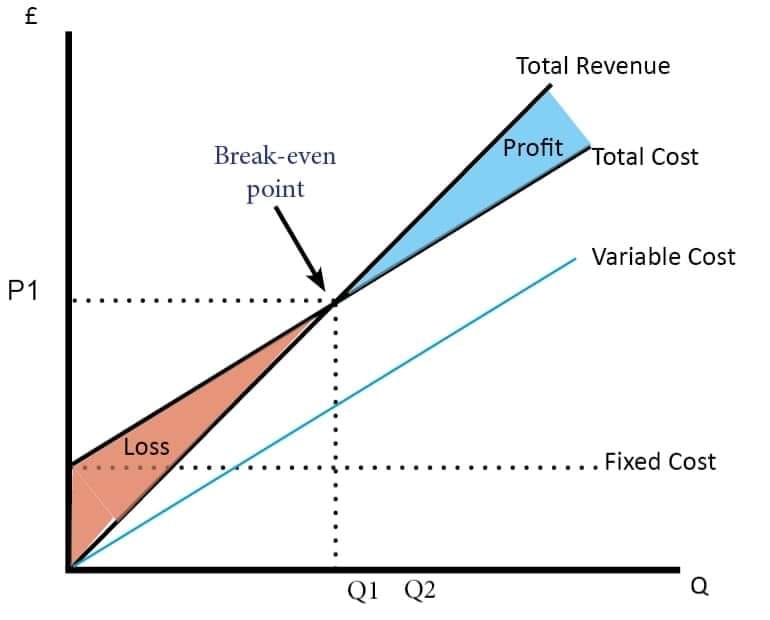
Computing Breakeven Quantity / Υπολογίζοντας το νεκρό σημείο πωλήσεων (ποσότητα) A canoe company sells paddles for $20 each. The unit variable cost is $15, and the fixed costs are $3000. How many paddles must be sold to breakeven? Μια εταιρία που φτιάχνει κανό, πουλά τα κουπιά με τιμή $20 το τεμάχιο. Το μεταβλητό κόστος παραγωγής είναι $15, και τα σταθερά κόστη είναι $3000. Πόσα κουπιά πρέπει να πουλήσει για να μην έχει ούτε κέρδος ούτε ζημιά (νεκρό σημείο πωλήσεων); Solution / Λύση Step 1 (Βήμα 1) Unit Selling Price (Τιμή Πώλησης Τεμαχίου) $20 – Unit Variable Cost (Μεταβλητό Κόστος Τεμαχίου) $15 = Gross Profit Margin (Μικτό Περιθώριο Κέρδους) $5 Step 2 (Βήμα 2) Fixed Costs (Σταθερά Κόστη) $3000 / Gross Profit Margin (Μικτό Περιθώριο Κέρδους) $5 = 600 paddles must be sold to breakeven (600 κουπιά πρέπει να πουληθούν για το νεκρό σημείων πωλήσεων) Equation for calculating GPM %…


Μετατροπή ποδιών σε μέτρα Feet Meter Formula for column Meter 20,00 6,10 =CONVERT(A5;”ft”;”m”) Μετατροπή βαθμών Φαρενάιτ σε Κελσίου Degree Fahrenheit Degree Celsius Formula for Degree Celsius 100,00 37,78 =CONVERT(D5;”F”;”C”) Μετατροπή ιπποδύναμης (HP) σε βατ (Watt) HP Watt Formula for column Watt 55,00 41013,49 =CONVERT(G5;”HP”;”W”)